Originally published October 2021.
Knowing what to ask is the trick to getting the right answer.
In The Hitchhiker’s Guide to the Galaxy, a supercomputer called Deep Thought is asked to answer the Ultimate Question of Life, The Universe and Everything. After 7.5 million years, Deep Thought reports back that the answer is 42. When questioned, Deep Thought points out that the answer seems meaningless only because it was not clear what the question was.
Calculating real estate risk can produce a similarly unclear answer for the people who asked for it and usually requires further clarification.
To provide a clear answer, a fund risk measure should quantify the likelihood of delivering an investment objective and of falling below a minimum level of return.
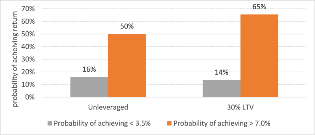
To illustrate, if the expected unleveraged return of a fund is 7% and the standard deviation is calculated as 3.5%, then the probability of achieving a 7% target rate of return is 50%, with a 16% chance of falling below a fund return of 3.5%.
Comparisons of these likelihoods can then be made to those for different portfolio structures, when adding leverage or for different funds. In our illustration, for example, adding leverage of 30% at an interest rate of 235 basis points increases the expected return to 9%, which boosts the likelihood of achieving the 7% target rate of return to 65% and reduces the chance of falling below 3.5% to 14%.
Chart 1: fund risk

Having a clear answer is one thing, ensuring confidence in the answer is another. The first way to engender confidence is to be transparent as to the calculations.
Future expected returns in any sector depend upon assumptions for growth, capital costs, vacancies, irrecoverable costs and price movements.
Future returns = Initial yield + growth – capital costs – vacancies – irrecoverable costs + yield change*
*Depreciation is captured in the growth, capital costs and yield change assumptions.
To illustrate, if the initial yield is 5% and average vacancies and irrecoverable costs are both 15% of income, then net operating income is reduced to 3.5%. Deducting capital costs of 1.0% pa, -0.5% for yield movement and adding growth of 2.5% would generate an expected return of 4.5% pa.
The outcomes for vacancies (which will predominantly drive irrecoverable costs) are the product of lease events: propensity to renew, propensity to break, tenant default and letting periods.
Table 1: illustrative market assumptions (research question – how do these expectations vary by sector?)

Listing expectations for each of the drivers of return allows an investor to see (and challenge) what the expected returns are based on. It is rare to see new fund launches being so open about their assumptions.
An additional benefit to the manager is that the outcomes can then be tracked against expectations, creating a ‘feedback loop’ to detect unexpected outcomes.
Typically, the inputs to individual asset plans (growth, letting periods, etc) are independently adjusted by the asset manager. While these plans are essential for asset management, the aggregate assumption for each of the performance drivers would then be an output of the modelling process. The danger is that the process is calculating the equivalent of six * nine (‘The Question’ imprinted in Arthur’s brainwaves in The Hitchhikers Guide to the Galaxy), especially if there is a tendency towards optimism in the individual property assumptions.
The problem is compounded when using the asset business plans to estimate fund risk.
The volatility of each sector return is due to variations in the outcomes for each of the drivers between strong and weak market conditions (defined as +/- one standard deviation).
To illustrate, let us assume that in strong market conditions rents grow in a sector by 7.5% pa, capital costs are 1% pa, irrecoverable costs and vacancies are 10% and yield change adds 1% to values. This generates an expected return of 11.5% pa. In weak market conditions, let us assume that rents fall by -2.5% pa, vacancies and irrecoverable costs rise to 25% of income and a yield rise reduces values by an equivalent of -2.5% pa, reducing the return to -2.5% pa.
The range from strong to weak market conditions can be used to estimate market risk. In addition to the market risk, individual fund properties will perform differently to their sector average based on the outcomes of individual lease events and the natural variation in growth and letting periods across properties.
Table 2: market assumptions in strong and weak market conditions (research question – how do the inputs vary in strong and weak market conditions in different sectors?)

Estimating individual property specific risk using hand-crafted asset business plans is possible, but it may seem to take 7.5 million years.
It is simpler and more transparent to adjust the fund risk estimate using average levels of specific risk in each sector. Total fund specific risk is then estimated using the number of properties in each sector.
To illustrate, the table below shows the figures for a fund of 45 properties that we recently analysed. The fund had a mix of core properties and developments with a spread of mostly retail parks and standard industrials. For a 10-year return horizon, roughly two-thirds of the total portfolio risk was estimated as structural and one-third due to undiversified specific risk.
Table 3: adding specific and market risk, illustration

Of course, it is possible that concentration risks emerge in a portfolio, such as a cluster of lease expiry dates, which will raise specific risks. These concentration risks should be monitored, as they can occur unexpectedly through the normal management of a portfolio.
Modelling fund risk based on individual asset business plans is a time-consuming exercise creating results that generate more questions than answers. Modelling fund risk as a separate exercise, using transparent inputs for sector volatility and specific risk, saves time and produces a transparent measure of risk.


